Bayesian Optimisation is a hyper-parameter tuning approach which usually adopts the Gaussian process as a surrogate model. Its acquisition functions Probability of Improvement (PI) and Expected Improvement (EI) are calculated with respect to current optima. In practice, The evaluations on loss function may contain noise at sampling positions, i.e. the loss function is noise corrupted. We can take noise into account by calculating the probability of improvement and expected improvement with respect to the posterior mean and variance at the current optima found. A white kernel should be added to the Gaussian Process kernel to fit the noise. Implementations in GitHub repo and tutorial.
Mathmatics
Probability of improvement (PI) and expected improvement (EI) are calculated with respect to the current optima \(\tilde{y}\). In some cases, each evaluation of the loss function has Gaussian noise \(y_i \sim \mathcal{N}\!\bigl(f(\mathbf{x})_i,\sigma_y^{2}\bigr)\). We modify PI & EI under the assumption that all observations—including the current optimum—contain noise. The two criteria are therefore computed with respect to the GP posterior mean \(\mu(\tilde{\mathbf{x}})\) and variance \(\kappa(\tilde{\mathbf{x}},\tilde{\mathbf{x}})\) at the optimum parameter setting \(\tilde{\mathbf{x}}\).
To learn the observation noise we add a white-noise kernel to the original Matérn kernel of the GP, which enables faithful uncertainty quantification at the sampled locations. Let \[ \rho \;=\; \sqrt{\kappa(\mathbf{x},\mathbf{x}) + \kappa(\tilde{\mathbf{x}}, \tilde{\mathbf{x}})\;-\;2\,\kappa(\mathbf{x},\tilde{\mathbf{x}})}. \] The modified acquisition functions become
\[
\text{Modified PI:}\quad
a_{\text{MPI}}(\mathbf{x}) \;=\;
\Phi\!\left(
\frac{\mu(\tilde{\mathbf{x}})-\mu(\mathbf{x})}{\rho}
\right)
\]
\[
\text{Modified EI:}\quad
a_{\text{MEI}}(\mathbf{x}) \;=\;
\Phi\!\left(
\frac{\mu(\tilde{\mathbf{x}})-\mu(\mathbf{x})}{\rho}
\right)
\bigl[\mu(\tilde{\mathbf{x}})-\mu(\mathbf{x})\bigr]
\;+\;
\phi\!\left(
\frac{\mu(\tilde{\mathbf{x}})-\mu(\mathbf{x})}{\rho}
\right)\rho
\]
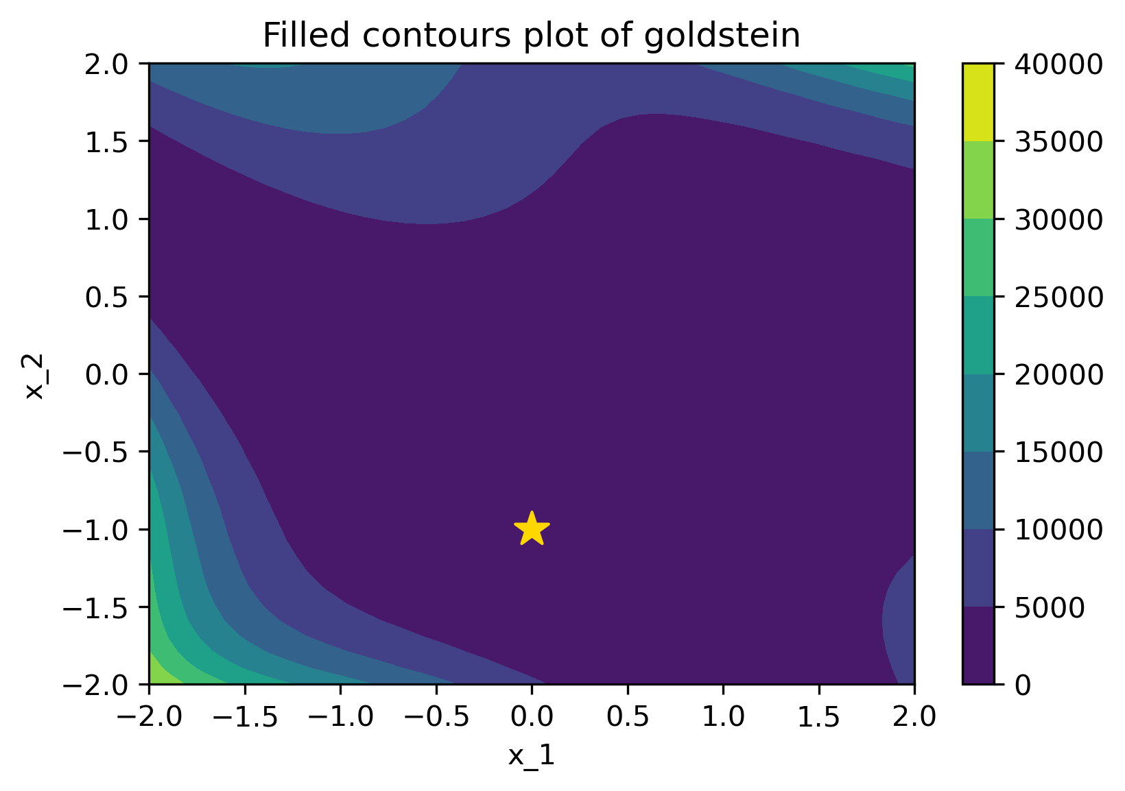
Below is a comparison of PI (left) and MPI+white kernel (right) optimizing on noise corrupted Goldstein-Price Function.
| Objective Loss function | Searching with PI | MPI+white kernel |
|---|---|---|
|
|
|
Publication: Huabing Wang, Modifications of PI and EI under Gaussian Noise Assumption in Current Optima . 2022